What you want to know (but dare to ask) about Conjunctive Query Processing

Abstract

Conjunctive Query (CQ) is a critical operation in OLAP databases. In this article, we examine traditional CQ processing methods, starting from binary join techniques, and discuss their limitations when scaling to multi-relation queries and complex patterns. We introduce several binary join processing models and analyze the trade-offs between parallelism and memory usage. Furthermore, we discuss the size bound of CQ, explaining why pure join planning may have bad worst case behavior, and we then exploring Worst-Case Optimal Join (WCOJ) methods and their variants. Finally, we give a introduction on free join, a unified theoretical framework for CQ processing.

Keywords: Conjunctive Query, Binary Join, Worst-Case Optimal Join, Free Join

1. Conjunctive Queries (CQs)

Conjunctive queries are a fundamental category of database queries in which the result is defined by a conjunction (logical AND) of conditions. For simplicity, we express conjunctive queries using Horn-clause syntax. A Horn clause consists of a rule in the form

where the head H is derived if all body clauses B1..n are satisfied. In this formulation, each clause corresponds to a database table, and each logical variable within a clause represents a column in that table. When a logical variable appears in multiple body clauses, it indicates that the corresponding tables are joined together on the columns that share that variable. In relational algebra terms, a Horn clause–based conjunctive query is equivalent to a select–project–join query.

foobar(a, b) :- foo(a, b), bar(b, c).

Semantically equal to $\Pi_{a,b}(\textit{foo} \bowtie_{b} \textit{bar})$ in relational algebra. For additional background and formal definitions, see the article on Wikipedia (Wikipedia).

1. Binary Join

Efficient join algorithms are crucial for quickly processing conjunctive queries. When a CQ involves only two relations, traditional binary join algorithms, such as hash join and sort-merge join, can be applied directly. For example, consider the foobar query mentioned above. A hash join implementation in pseudocode might look like this:

for (a, b) in foo {
	let bar_rows = bar[b];
	for (b, c) in bar_rows { // bar indexed on the column named "b"
		foobar.insert((a, c));
	}
}

We first build a hash map on the column b in the bar relation, which maps each b value to all corresponding tuples. Next, we scan through the tuples in the foo relation; for each tuple in foo, we query bar’s hash map using its b value, thereby retrieving and materializing all matching tuples from bar into bar_rows. Finally, for each tuple in bar_rows, we project and construct a new foobar tuple.

Note: In the literature, the scanned relation (foo in this case) is often referred to as the outer relation, while the indexed relation (bar) is called the inner relation.

Real-world CQs usually consist of multiple input relations. For example considering following CQ:

foobar(a, c, d) :- foo(a, b), bar(b, c), baz(a, d).

To process this query using binary joins, we break it into a sequence of two binary joins: first, join foo and bar; then, join the intermediate result with baz.

In pseudocode, this process looks like:

let tmp = vec![];
for (a, b) in foo {
	let bar_rows = bar[a];
	for (b, c) in bar_rows {
		tmp.insert((a,c));
	}
}
for (a, c) in tmp {
	let baz_rows = baz[a];
	for (a, d) in baz_rows {
		foobar.insert((a,c,d));
	}
}

In this processing model, the primary computational effort lies in executing nested loops. The memory overhead mainly originates from two parts: the temporary buffer tmp used to materialize the intermediate join, as well as the arrays bar_rows/baz_rows created inside the loops to materialize the projected tuples.

Join Plan

Besides joining foo and bar first, alternative join orders exist for processing the three-way join. For example, we can decompose the query into two intermediate joins—computing $(\textit{foo} \bowtie_{b} \textit{bar})$ and $(\textit{foo} \bowtie_{a} \textit{baz})$ separately—and then joining these intermediate results. These decompositions are known as binary join plans, which break a k-way join into a sequence of binary joins.

A common isomorphism is treat each relation as node, shared logic variables as edges, then these different ways of join will form different type of graphs. The first ad-hoc sequential plan forms a left-deep tree (called left-deep linear plan), while the alternative plan forms a more branched structure called a bushy plan.

Note: Some plan graphs may contain cycles. In this section, we focus on acyclic, tree-shaped join graphs, and we will discuss cyclic graphs later.

The efficiency of a given join plan heavily depends on the size of the intermediate results produced by each pairwise join. In a three-way join, a smaller intermediate result from the first join not only reduces memory overhead by requiring a smaller buffer but also minimizes the amount of work needed in the subsequent join.

For tree-shaped join graphs, although different join plans may exhibit varying topologies, their processing can be approached similarly. Both bushy and left-deep plans can be efficiently executed via a bottom-up traversal of the join tree, converting joins into semi-joins(i.e. a join using select and where clause), a technique established by Yannakakis in the 1980s (Yannakakis). Consequently, optimizing left-deep plans is generally considered sufficient for achieving high performance, thereby simplifying the overall join processing strategy.

3. Memory or Parallel?

Pipelining

In the earlier pseudocode, we stored the intermediate result of joining foo and bar in a vector tmp. However, in real-world queries—such as when foo represents the edges of a large social media graph—this temporary result can be enormous, leading to significant memory overhead.

To avoid materializing such large intermediate results, a classic approach is to pipeline the join operations. In pipelining, the output of one binary join is immediately fed into the next binary join operation without being fully stored. The following pseudocode illustrates this approach:

for (a, b) in foo {             // using openmp pfor
	for (b, c) in bar[a] {
		for (a, d) in gez[a] {
			foobar.insert((a,c,d));
		}
	}
}

This pipelined model relies on a data structure that supports range probing on all tuples sharing the same join attribute value(such as a hash map, B-tree, or trie) combined with pointer-like access to an internal subset of the relation via an iterator design pattern. This processing model was firsted introduced in a database optimization system called Volcano (Graefe and McKenna), therefore also known as volcano or iterator model (Palvo) in some other literatures.

In addition to its efficient memory usage, the pipelining model can be readily accelerated on multicore CPUs. To enhance pipelined processing, the workload can be divided based on the outermost loop. By evenly partitioning the tuples in foo across available threads, each thread processes a subset concurrently, thereby boosting overall performance.

Data Skew

However, data skew may cause the scaling problem in a pipelined model. For instance, in a large social media graph, some influential nodes may have hundreds of times more followers than other nodes. When such a graph serves as the outer relation in a multi-input relation CQ, the thread processing the influential node will have to handle significantly more work compared to threads processing less-connected nodes.

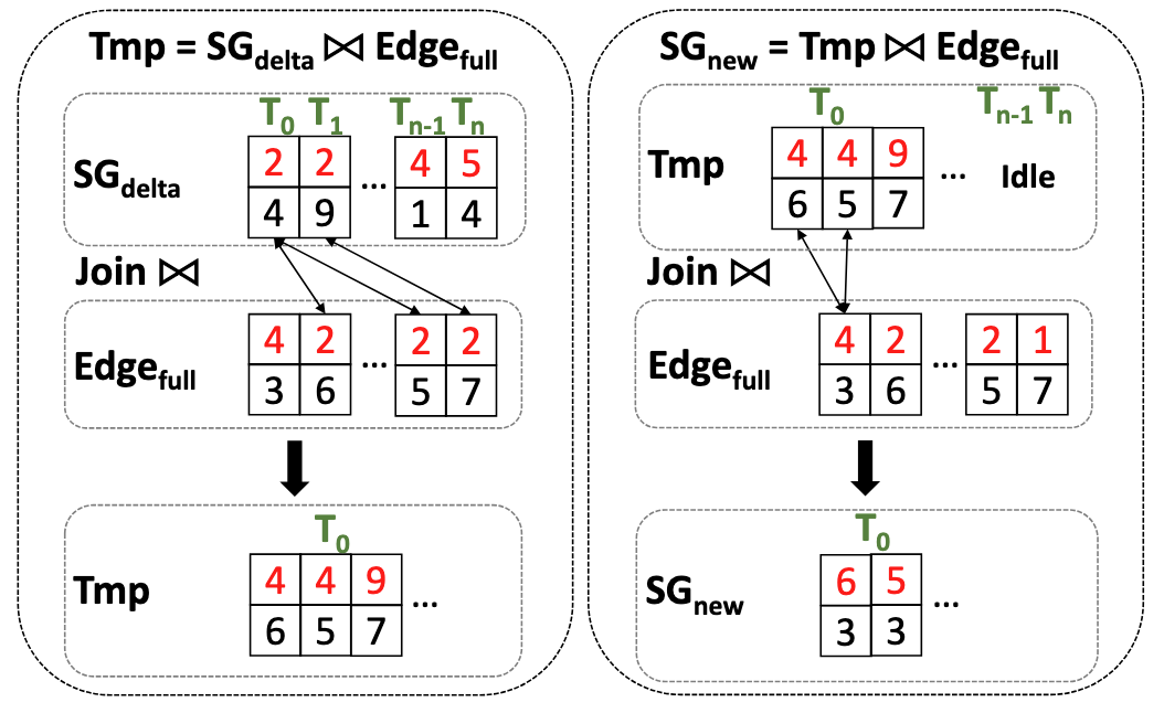
For example, in the figure above, many edge tuples share the indexed value 2. As a result, the outer-most relation tuples such as (2,4) and (2,9), processed by threads $T_0$, need to join three tuples sharing the join attribute value 2. Consequently, in the inner loop of the pipelined model (illustrated on the right side of the figure), thread $T_0$ must continue processing join. Meanwhile, threads $T_{n-1}$ and $T_n$ remain mostly idle in the inner loop because the outer tuples they scan have no matching inner tuples.

This imbalance in join processing makes it difficult to scale pipelined join operations on massively parallel hardware and hinders adaptation to SIMD-based architectures, such as GPUs and AVX-supported CPUs.

Recalling the first temporary materialization approach we discussed, while it does incur extra memory overhead, the key advantage is that the scanning loops over foo and the temporary result (tmp) operate independently. This decoupling means that even if data skew occurs in foo, it doesn’t disproportionately load any single thread during the scan over tmp. As a result, the overall workload is more evenly balanced across threads, minimizing the risk of thread idling due to uneven data distribution. And thus this materialization approach adopted by some GPU/supercomputer based parallel CQ query engines.

Vectorization

Vectorization is an intermediate approach that combines the benefits of pipelining and full materialization. Instead of materializing every intermediate tuple, vectorized processing handles only a limited number of tuples at a time, grouping them into batches. Similar to pipelining, it relies on data structures that support range probing; however, each move of the iterator now returns a batch of tuples instead of a single tuple. This approach helps reduce memory overhead while still enabling efficient batch processing and improved cache utilization.

In pseudo code:

let cur_foo = foo.begin();
let cur_bar = bar.begin();
let BATCH_SIZE = ...;
while cur_foo != foo.end() &&
      cur_bar != bar.end() {
	let tmp[BATCH_SIZE];
	let tmp_cnt = 0;
	pfor (a, b) in cur_foo.next() {
		if let None = *cur_bar {
			cur_bar = bar[a];
		}
		for (b, c) in cur_bar.iter() {         // imbalance
			if tmp_cnt < BATCH_SIZE {
				let pos = atomicAdd(tmp_cnt);
				tmp[pos] = (a,c);
			} else {
				cur_foo = ...
				cur_bar = ...
			}
		}
	}
	pfor (a, c) in tmp {
		for (a, d) in gez[a] {                 // imbalance
			foobar.insert((a,c,d));
		}
	}
}

Using a fixed-size temporary buffer allows vectorized processing to control memory overhead effectively. In this model, the join operations for $\textit{foo} \bowtie_{b} \textit{bar}$ and $\textit{tmp} \bowtie_{a} \textit{gez}$ are decoupled, so workload balance is maintained, and each operation does not adversely affect the other. The pre-allocated fixed-size buffer also enables lock-free access, avoiding the need for a locking parallel append operation on a dynamically sized vector.

Despite these benefits, for architectures such as SIMD/SIMT where each thread must execute the same (or nearly the same) amount of work, above processing approach may still be insufficiently balanced. For example, in GPU-based databases, the inner loops of the parallel pfor constructs can experience varying workloads when data is severely skewed. Recent work (see (Lai et al.)) suggests that fixing the batch size to be similar to the thread count and allowing each thread to return as soon as all threads have found at least one matching tuple in the join could help address this imbalance when executed on datacenter GPUs.

Vectorized processing is considerably more complex than the previously discussed processing model, particularly when it comes to details such as partitioning batches, selecting appropriate batch sizes, swizzling, and adapting to the memory hierarchy of specific hardware. This remains an open research question, especially in the context of modern data parallel hardware systems.

4. Query Size Estimation: Bound of CQs

The pseudocode for conjunctive query (CQ) processing shows that the running time of a CQ query is polynomial, as it essentially involves a series of nested loops over the candidate relations. Consequently, the overall running time is generally bounded by the sizes of the input relations. In following foobar query, assume foo has size $N_1$ and bar has size $N_2$ , baz has size $N_3$:

foobar(a, b, c, d) :- foo(a, b), bar(b, c), baz(c, d).

In the worst-case scenario, suppose there is only a single distinct value for the join attribute b in both foo and bar. In this case, every tuple in foo will match every tuple in bar, meaning the join of foo and bar could produce up to $N_1 \times N_2$ tuples. When this intermediate result is subsequently joined with baz, the upper bound on the result size becomes $N_1 \times N_2 \times N_3$. Here, the hash table built on bar provides no benefit because the join cannot filter out any tuples, so the running time is fully dependent on the input sizes.

Standard left-most linear binary join planning analysis suggests that “the size bound of a CQ equals the multiplication of all input relations.” However, tighter bounds are achievable with more optimal query planning strategies. Consider the following triangle query:

foobar(a, b, c) :- foo(a, b), bar(b, c), baz(a, c).

In this query, the relation baz does not introduce any new logical variables, as both a and c have already appeared in earlier atoms. Consequently, the output size is not the full product of the input relation sizes; instead, it is determined by the largest of the pairwise joins among the three relations. A tighter theoretical upper bound for this query is:

This bound is polynominal smaller than the naive cubic upper bound.

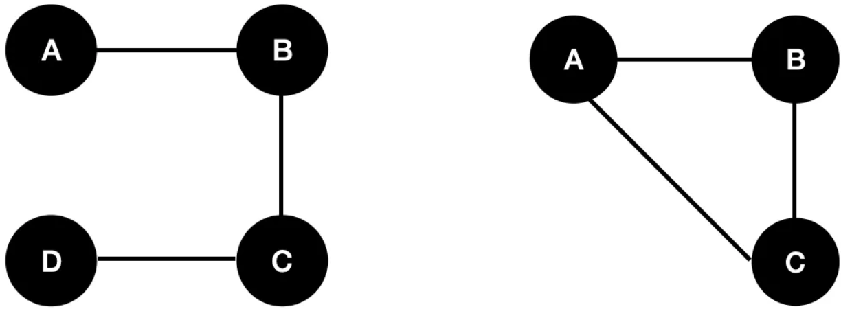
A natural way to reason about how each relation and column contributes to the CQ is by constructing a query graph: nodes represent logical variables (i.e., column names), and edges represent the relations. In this model, worst-case join planning can be seen as an edge cover problem, where the goal is to identify a minimal set of vertices that touches every edge. For example, for two foobar query graphs we show earlier in this section, the first one might use the vertex set ${A, D, C}$ to represent the worst case for the first query, while the vertex set ${A, B}$ will be sufficient for the second query, indicating that the worst-case output size is dominated by fewer variables.

• Note:

  For relations with an arity greater than two, these can be modeled as hyperedges in a hypergraph, and the overall discussion remains analogous. For simplicity, this article focuses exclusively on binary (two-arity) relations.

Therefore, the optimal join processing strategy for a triangle query should focus on processing only the unique values of a and c in foo and baz. In contrast, row-wise join processing tends to repeatedly handle different rows that share the same a and c values, particularly when data skew is present. This observation indicates that, to reach the optimal bound, it is necessary to abandon row-wise join processing in favor of a column-wise approach, which enables rapid selection of all unique column values involved in the query.

AGM Bound

In 2013, Atserias, Grohe, and Marx demonstrated that a tighter worst-case bound (AGM bound) (Atserias et al.) related to geometric mean of input relation sizes exists for conjunctive queries under select-join planning. To derive this bound, we refine our graph model from a simple edge cover to a more fine-grained fractional edge cover. In this model, each relation (or vertex) is assigned a fractional weight that represents the proportion of tuples contributing to the join result, with the constraint that for every logical variable (edge) in the query, the sum of the weights of the connected relations is at least 1. Formally :

The fractional edge of a conjunctive query $q$ is a vector $u$, which assign a weight $u_j$ to vertex $R_j$ (representing a relation), such that for every edge (representing logical variable) connect to it

The AGM bound is derived by linking fractional edge covers to entropy inequalities. Assume the query result $q(D)$ is a uniformly distributed on random variable $X=(X_a)_{a \in \textit{vars}(q)}$. It’s entropy is:

For uniform distributions, this simplifies to:

According to Shear’s lemma https://en.wikipedia.org/wiki/Shearer%27s_inequality, which generalizes entropy bound to overlapping marginal distribution, we derive:

Exponentiating both sides yields the AGM bound:

The AGM bound is tight, meaning there exist database instances where equality holds. Formally,

The tightness of this bound allow us to use linear programming for finding the optimal solution

Using languages of constraint satisfication problem, it can be formally written as:

The optimal fractional edge cover number of the query, denoted as $\rho^*(Q)$, is then used to define the AGM bound. Specifically, if the total number of tuples in the database is $\lvert D \rvert$, the worst-case output size of the query is bounded by:

Specifically, consider in the triangle join we shown before, where the size of each input relation is $N$; rather than the join output being bounded by $O(N^3)$, their result implies that the worst-case output size can be bounded by

(Detail proof is shown in (Atserias et al.).)

5. Worst Case Optimal Join

Inspired by AGM bound, Hung Q. Ngo, Christopher Re and Atri Rudra purpose a generic framework (missing reference) for designing worst case optimal join. Their algorithm can be described using the following pseudocode:

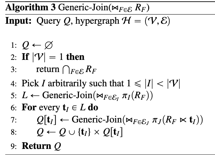
At each recursion level, the algorithm selects a join variable—typically chosen based on heuristics such as frequency of occurrence across relations. It then projects the selected variable from all participating relations and computes the intersection of these value sets to determine all possible assignments to that logical variable. For each intersected value, the algorithm grounds the query accordingly and recursively applies the same process to the partially grounded query. This recursion continues until all variables in the query are bound, yielding a complete join result. This project-intersect-join pattern, this match the suggestion of original AGM paper.

For a known query such as the triangle query, we can unroll the recursive process of the generic worst-case optimal join (WCOJ) algorithm as follows:

for a in foo.a ∩ baz.a:
	foo_tmp = foo[a]; baz_tmp = baz[a];
	for b in foo_tmp.b ∩ bar.b:
		bar_tmp = bar[b]
		for c in baz_tmp.c ∩ bar_tmp.c:
			foobar(a, b, c)

Delayed Materialization

One notable thing of the generic WCOJ algorithm is that it requires allocating temporary buffers at each level of the recursion (or nested for-loop) to store intermediate results, the partially grounded tuples. This introduces more memory overhead, when compared to traditional left-deep binary joins, where intermediate results are often pipelined or materialized in global buffer. If we use the same data structures for both storage and join processing (as is common in left-deep plans), this memory pressure can severely impact performance. A common solution is using prefix trie as relation data structure.

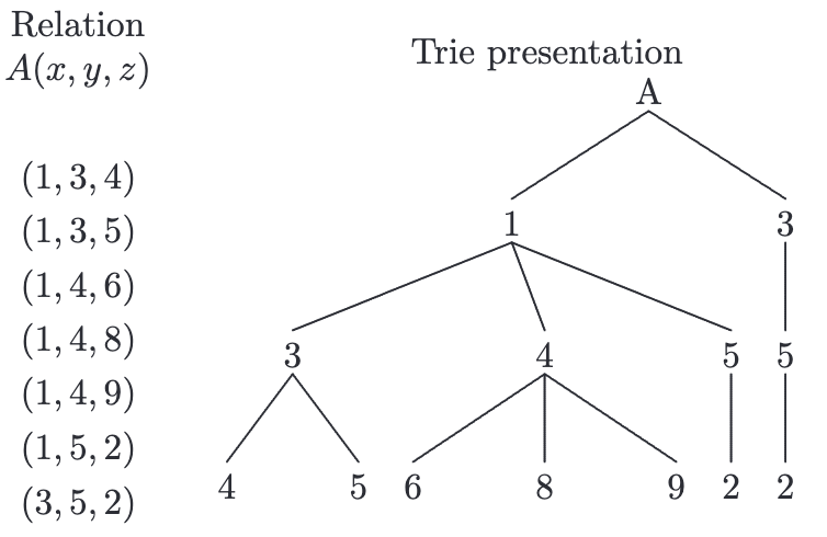
For example in above relation A stored in trie, operation A[1] can now be implemented as finding the pointer of sub-tree rooted at value one and instead of temporary buffer we only need store a single pointer.

A key downside of trie-based relation storage is that it makes random access and iteration over entire tuples—which are essential in many traditional, row-oriented database systems—more difficult and less efficient. However, this limitation is less problematic in the context of WCOJ. Fortunately, WCOJ algorithms operate exclusively on individual columns, performing set intersections, projections, and filters, rather than full tuple-level operations. This column-oriented access pattern aligns well with our discussion in Section 4: achieving tighter output size bounds fundamentally requires column-oriented processing rather than traditional row-oriented execution.

• Note:

  There has been a long-standing discussion in the database community regarding column-oriented vs. row-oriented systems (Abadi et al.). The choice of storage model depends on several factors, including hardware architecture, data characteristics, and query patterns. A full exploration of this topic is beyond the scope of this article.

Leapfrog triejoin

In generic WCOJ algorithms, temporary storage is needed not only for grounding partially bound tuples but also for computing set intersections at each level of recursion. To reduce memory overhead, we can borrow techniques from traditional left-most binary join processing by adopting a pipelined, iterator-based approach. This strategy changes the paradigm from “intersect all, then process” to “find one intersection, process it, then move to the next,” thereby avoiding the need to materialize large intermediate intersection sets.

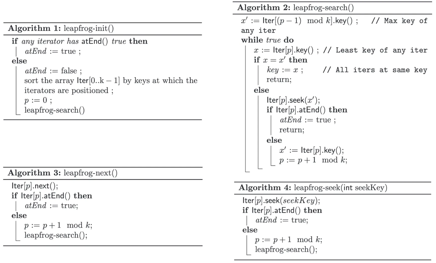
An implementation of this idea is Leapfrog Triejoin (LFTJ) (Veldhuizen), introduced by Todd L. Veldhuizen and used in the commercial system LogicBlox. LFTJ is specifically designed for scenarios where all column values are integers and each relation is indexed using a sorted trie. In such tries, each level corresponds to a join variable, and the children (subtries) of every node are kept in sorted order. Below pseudo code describe the LFTJ using iterator-model style:

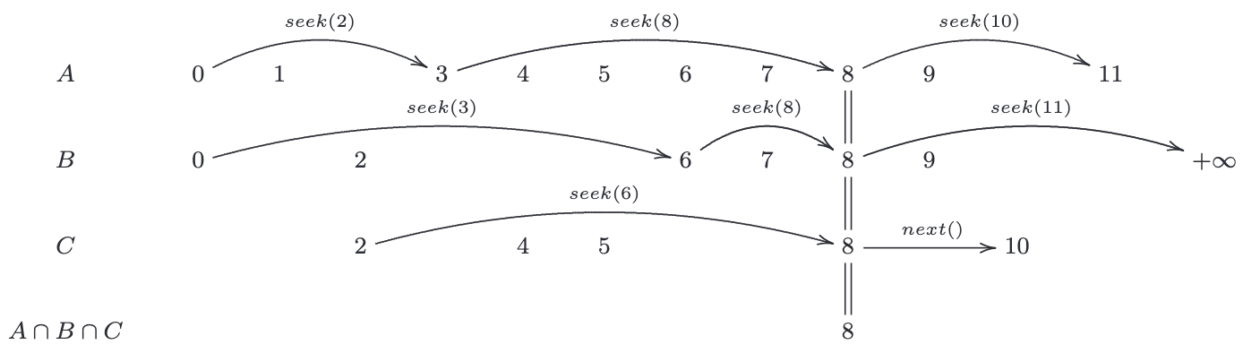
Below is a concrete example illustrating the algorithm’s operation. Initially, the algorithm initializes an iterator over each input relation’s join column. In this example, the iterators for relations A, B, and C are positioned at 0, 0, and 2, respectively. The algorithm then determines the candidate join value by computing the maximum of these initial values as possible lower-bound of next joined value, which is 2—this value is currently held by relation C. Next, the algorithm uses the linear probing function (leapfrog-seek) to search for the candidate value 2 in another relation—in this case, relation A is arbitrarily chosen. During the search in relation A, it is found that 2 is not present; instead, the iterator advances to the smallest value greater than 2, which is 3. With 3 as the new possible lower-bound of next joined value, the algorithm then repeats the search in relation B.This process of advancing the iterators continues until a candidate join value (in the example, 8) is present in all relations. When such a value is found, it confirms that the value lies in the intersection of all join columns, allowing the algorithm to proceed with the inner loop of the generic join operation.

Although LFTJ is a compelling algorithm for pipelining worst-case optimal joins, its reliance on sorted tries for relation storage can be limiting. While sorted tries support efficient sequential iteration, they impose an ordering constraint that can result in non-constant factor access during lookups. For systems that require truly constant-factor indexed value access, a hash-trie based algorithm is more appealing.

Free Join

Recall that we discussed three key techniques for accelerating the processing of a worst case optimal CQ:

1. Using column-oriented join (as seen in generic WCOJ).
2. Late intermediate result materialization (via trie-based relation storage).
3. One join result per iteration (through pipelining, as in LFTJ).

A natural question then emerges: Is there a unified framework that could enable all of these approaches? Recent work by Remy Wang and Max Willsey proposes answer to this question through a framework called free join (Wang et al.).

Free join decomposes a query into multiple subatoms, which are simply subsets of a relation’s columns. Formally:

Given a relation schema $R(x_1, x_2, …)$, a subatom is the form $R(x_i, x_j, …)$ where ${x_i, x_j,…} \subseteq {x_1, x_2, …}$.

A free join over a set of schemas is a sequence of groups, where each group is a list of subatoms. Formally,

where each of $R_i(x_i), R_j(x_j), R_k(x_k),…$ is a subatom over a the schema of $R_i, R_j, R_k, …$ respectively.

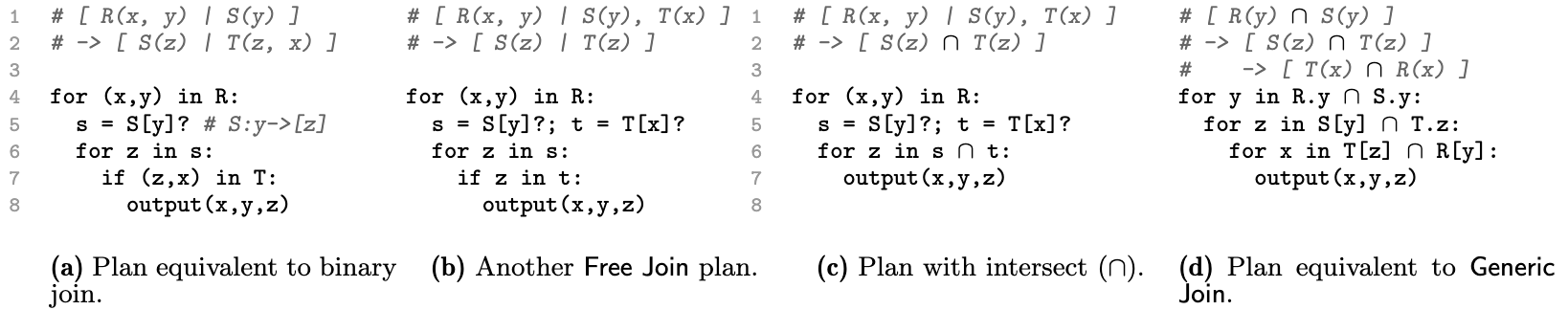
To interpret a free join plan, simply treat each bracketed group [] as a loop level. Within each level, iterate over the first subatom of the group, and use the scanned value to ground (or filter) and look up the remaining subatoms. For example, the triangle query with WCOJ optimizations can be represented in pseudocode as follows:

One bonus contribution of the original Free Join paper is that it also presents an algorithm for implementing the join plan using a novel data structure called the Lazy Generalized Hash Trie (LGHT). Similar to how the sorted trie enables the pipelining of worst-case optimal joins in LFTJ, LGHT makes it possible to fully pipeline hash-based WCOJ.

What’s Next ?

In this article, we have explored a wide range of processing algorithms for conjunctive queries, but most of them only run on single CPU system—especially worst-case optimal join techniques. However, scaling these methods to parallel processing environments remains a complex and open research question. Recent work on adapting worst-case optimal joins to parallel hardware (see (Wu and Suciu) (Lai et al.)) shows promising directions, though none of these approaches have matured for use in real-world databases. Besides this article, a recent extensive survey is (Koutris et al.), please check it out for more details on conjunctive query processing. I am also looking forward to discussing these developments and sharing my thoughts on parallelizing conjunctive query processing in future blog articles.

Reference

1. Wikipedia. Conjunctive Query. 2024, https://en.wikipedia.org/wiki/Conjunctive_query.
2. Yannakakis, Mihalis. “Algorithms for Acyclic Database Schemes.” VLDB, vol. 81, 1981, pp. 82–94.
3. Graefe, Goetz, and William J. McKenna. “The Volcano Optimizer Generator: Extensibility and Efficient Search.” Proceedings of IEEE 9th International Conference on Data Engineering, IEEE, 1993, pp. 209–18.
4. Palvo, Andy. Lecture Note of Andy Palvo on Multi-Way Join Algorithm. 2024, https://15721.courses.cs.cmu.edu/spring2024/notes/10-multiwayjoins.pdf.
5. Lai, Zhuohang, et al. “Accelerating Multi-Way Joins on the GPU.” The VLDB Journal, 2022, pp. 1–25.
6. Atserias, Albert, et al. “Size Bounds and Query Plans for Relational Joins.” SIAM Journal on Computing, vol. 42, no. 4, 2013, pp. 1737–67.
7. Abadi, Daniel, et al. “The Design and Implementation of Modern Column-Oriented Database Systems.” Foundations and Trends&#0174 in Databases, vol. 5, no. 3, 2013, pp. 197–280.
8. Veldhuizen, Todd L. “Leapfrog Triejoin: A Simple, Worst-Case Optimal Join Algorithm.” Proc. International Conference on Database Theory, 2014.
9. Wang, Yong Rong, et al. “Free Join: Unifying Worst-Case Optimal and Traditional Joins.” Proceedings of the ACM on Management of Data, vol. 1, no. 2, 2023, pp. 1–23.
10. Wu, Jiacheng, and Dan Suciu. “HoneyComb: A Parallel Worst-Case Optimal Join on Multicores.” ArXiv Preprint ArXiv:2502.06715, 2025.
11. Koutris, Paraschos, et al. “The Quest for Faster Join Algorithms (Invited Talk).” 28th International Conference on Database Theory (ICDT 2025), Schloss Dagstuhl–Leibniz-Zentrum für Informatik, 2025, pp. 1–1.